Heads up to readers: this is a long article with lots of code samples and interactive charts. If you're reading on a mobile device, you might want to save this one until you can get to a wider screen! It may take a while to load all the charts.
Introduction
This is a longish post about using a simple evolutionary algorithm in Python to create a strategy for playing the famous Prisoner's Dilemma game (actually, the version known as Iterated Prisoner's Dilemma, hereafter referred to as IPD). If you're not already familiar with the Prisoner's Dilemma, take a look at the first bit of the Wikipedia page and the section on Iterated Prisoner's Dilemma. You might also want to watch this short video and take a look at this blog post.
The impetus for this project was hearing about (and then working on a code sprint for) the Axelrod library at PyConUk 2015. Axelrod is a Python library which provides a framework for running IPD tournaments. This makes it very easy to play around with different strategies.
Strategies are implemented as classes which have a single method, strategy() which takes as its argument an opponent object, and returns an action. Actions are represented by C for cooperate and D for defect. For example, here's the famous Tit for tat strategy that won the original Axelrod tournament in 1980, which can be summarized as "co-operate on the first turn, then copy the opponent's last action":
def strategy(self, opponent):
    """This is the actual strategy"""
    # First move
    if len(self.history) == 0:
        return C
    # React to the opponent's last move
    if opponent.history[-1] == D:
        return D
    return C
As we can see, the player has access to its own history through the self.history variable and to the opponent's history though the opponent.history variable. Players can implement more sophisticated strategies by examining these variables, and they also have access to the length of the match. For example, when I first encountered the Axelrod library the winning strategy was called DoubleCrosser* and worked like this (edited slightly for clarity):
 def strategy(self, opponent):

    # if there is no history, then this is the first turn, so cooperate
    if not opponent.history:
        return C

    # if this is either the last or second-to-last turn, defect
    if len(opponent.history) > (self.tournament_attributes['length'] - 3):
        return D

    # if the opponent did not defect on any of the first six turns,
    # and we are not in the last 20 turns, cooperate
    if len(opponent.history) < 180:
        if len(opponent.history) > 6:
            if D not in opponent.history[:7]:
                 return C

    # if the total number of defections by the opponent is
    # greater than three, always defect
    if opponent.defections > 3:
        return D

    # failsafe; if none of the other conditions are true,
    # cooperate
    return C
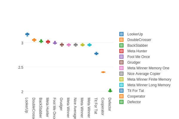
The library takes care of matching up players in pairwise combinations, running the tournament for a given number of turns, and keeping score. For the sake of convenience, scores are usually expressed as average score per turn. The best possible outcome for a given turn is that a player defects and their opponent cooperates giving a score of 5 in the standard payoff matrix, so that's the theoretical best average score per turn. The best strategies in the Axelrod library currently score around 3*. Here's a chart showing the ten best strategies, plus Tit for Tat, Cooperator, and Defector for reference:
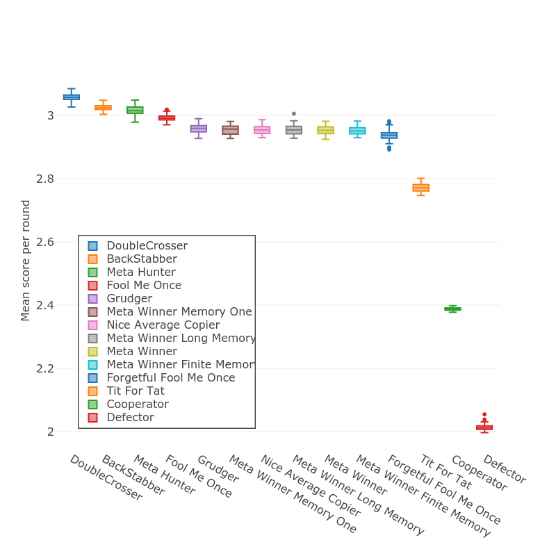
The reason that we're looking at a box plot here is that some of the strategies are stochastic, i.e. there's some random variation in the action they take. When calculating the scores, the Axelrod library takes care of running the tournament multiple times (100 by default) to get an average score for each strategy.
Using lookup tables to define a strategy
Many of the strategies in the Axelrod library choose their action based on what happened on the previous turn (or possibly earlier in the history). Tit for Tat is a good example; its action on a given turn depends entirely on the opponent's action on the previous one. We can think of this as a lookup table:
| Opponent's previous action | My action |
|---|---|
| Cooperate | Cooperate |
| Defect | Defect |
or, in Python, as a dict where the keys are opponent's previous action, and the values are my action:
lookup_table = {
    'C' : 'C',
    'D' : 'D'
}
If we wanted to write a strategy that used this lookup table to decide what action to take, we could just grab the opponent's last action from its history like this:
def strategy(self, opponent):
    lookup_table = {
            'C' : 'C',
            'D' : 'D'
        }

    # First move
    if len(self.history) == 0:
        return C

    # Get the opponent's last action
    last_action = opponent.history[-1]
    # Use it to look up my action
    my_action = lookup_table[last_action]
    return my_action
Notice that we still need a special case for the first turn; obviously if there is no history then we can't use the lookup table!
The nice thing about expressing a strategy in this was is that we can get different behaviours by changing the lookup table and leaving the strategy code exactly the same. In other words, the strategy is completely determined by the lookup table. For our current example, this isn't very exciting - given that there are only two possibilities for the dict key there are only three other strategies that we can describe: Cooperator:
# always cooperate
lookup_table = {
        'C' : 'C',
        'D' : 'C'
    }
, Defector:
# always defect
lookup_table = {
        'C' : 'D',
        'D' : 'D'
    }
, and Inverse Tit for Tat, which always does the opposite of the opponent's last action:
# do the opposite of my opponent's last action
lookup_table = {
        'C' : 'D',
        'D' : 'C'
    }
Things start to get interesting when we use the last two turns of the opponent's history as the key to the lookup table. Take a look at this table:
| Opponent's recent history | My action |
|---|---|
| Cooperate, Cooperate | Cooperate |
| Cooperate, Defect | Cooperate |
| Defect, Cooperate | Cooperate |
| Defect, Defect | Defect |
There are now four different possibilities (two for each turn) which allows us to express a more complex strategy. Here, we only defect if the opponent has defected twice in a row (this strategy is known as Tit for Two Tats). Here's the corresponding dict:
lookup_table = {
        'CC' : 'C',
        'CD' : 'C',
        'DC' : 'C',
        'DD' : 'D',
    }
In order to use this lookup table in a strategy() method, we need to get the opponent's last two actions and join them together to make a string, and we also need to decide what to do on the first two turns:
def strategy(self, opponent):

    lookup_table = {
        'CC' : 'C',
        'CD' : 'C',
        'DC' : 'C',
        'DD' : 'D',
    }

    # First two moves
    if len(self.history) < 2:
        return C

    # Get the opponent's last two actions
    opponent_actions = opponent.history[-2:]
    # Use it to look up my action
    my_action = lookup_table[opponent_actions]
    return my_action
We can extend this idea even further: what if we wanted to take into account our own history as well as our opponents? That gives us sixteen different possibilities (four for us multiplied by four for our opponent); here's what the first few rows of the table would look like:
| Opponent's recent history | My recent history | My action |
|---|---|---|
| Cooperate, Cooperate | Cooperate, Cooperate | ? |
| Cooperate, Defect | Cooperate, Cooperate | ? |
| ... | ... | ... |
And we can now think about even more complex rules. For example, if we defected and the opponent didn't retaliate, then defect again:
| Opponent's recent history | My recent history | My action |
|---|---|---|
| ... | ... | ... |
| Cooperate, Cooperate | Defect, Defect | Defect |
| ... | ... | ... |
Or we might want a rule that we never defect more than twice in a row:
| Opponent's recent history | My recent history | My action |
|---|---|---|
| ... | ... | ... |
| Cooperate, Cooperate | Defect, Defect | Cooperate |
| Cooperate, Defect | Defect, Defect | Cooperate |
| Defect, Cooperate | Defect, Defect | Cooperate |
| Defect, Defect | Defect, Defect | Cooperate |
| ... | ... | ... |
To write this lookup table as a dict, we'll create a tuple consisting of our last two actions, and our opponent's last two actions, and use that as the key. So the key/value pairs for the rule in the table above looks like this:
lookup_table = {
    ...
    ('CC', 'DD') : 'C',
    ('CD', 'DD') : 'C',
    ('DC', 'DD') : 'C',
    ('DD', 'DD') : 'C',
    ...
}
Mathematically-inclined readers will have noticed that as we increase the number of keys in the lookup table dict, the number of possible strategies we can describe increases rather rapidly. Each key can result in two possible values (cooperate or defect), so for n keys there are 2^n possible lookup tables. The above example has 16 keys, which gives us 65,536 different strategies.
Finally, let's add another factor to our lookup table: the opponent's first two moves. This gives us the ability to implement rules like "if we defected and the opponent didn't retaliate then defect again, but only if the opponent started off by cooperating":
| Opponent's first actions | Opponent's recent history | My recent history | My action |
|---|---|---|---|
| ... | ... | ... | ... |
| Cooperate, Cooperate | Cooperate, Cooperate | Defect, Defect | Defect |
| Defect, Defect | Cooperate, Cooperate | Defect, Defect | Cooperate |
| ... | ... | ... | ... |
The keys for our lookup table dict are now 3-tuples consisting of the opponent's starting actions, the opponent's recent actions, and our recent actions:
lookup_table = {
    ...
    ('CC', 'CC', 'DD') : 'D',
    ('DD', 'CC', 'DD') : 'C',
    ...
}
This key structure gives us 64 different keys and about 10^18 different strategies. If we're interested in finding the best strategy - i.e. the one that gives the highest average score per turn - we're going to need a way of exploring the strategies. On a reasonably modern desktop it takes around 3 seconds to score a single table* so an exhaustive brute-force search will take around 90 billion years. We're going to need something a bit more sophisticated.
Searching lookup table space to find good ones
To search for "good" strategies that use a 64-key lookup table, we need a way to quickly create a player object for a given dict. Here's a simplified version of the code*:
class LookerUp(Player):

    def __init__(self, lookup_table):
        self.lookup_table = lookup_table


    def strategy(self, opponent):
        # If there isn't enough history to lookup an action, cooperate.
        if len(self.history) < 2:
            return C

        # Get my own last two actions
        my_history = ''.join(self.history[-2:])

        # Do the same for the opponent.
        opponent_history = ''.join(opponent.history[-2:])

        # Get the opponents first two actions.
        opponent_start = ''.join(opponent.history[:2])

        # Put these three strings together in a tuple.
        key = (opponent_start, my_history, opponent_history)

        # Look up the action associated with that tuple in the lookup table.
        action = self.lookup_table[key]

        return action
The idea behind this strategy is that we can pass in a lookup table to the constructor to determine what strategy our player will play. For instance, here's Cooperator:
# this table actually has all 64 possible keys, not all shown
cooperator_table = {
    ('CC', 'CC', 'CC'): 'C',
    ('CC', 'CC', 'CD'): 'C',
    ('CC', 'CC', 'DC'): 'C',
    ...
    ('DD', 'DD', 'DC'): 'C',
    ('DD', 'DD', 'DD'): 'C'}
}

cooperator = LookerUp(cooperator_table)
We will also need a couple of utility functions to help us calculate the score for a given lookup table. Here's a function that will take two player objects, play a match between them, and return the average per-turn score of the first one:
def score_single(me, other, iterations=200):
    """
    Return the average score per turn for a player in a single match against
    an opponent.
     """
    g = axelrod.Game()
    for _ in range(iterations):
        me.play(other)
    return sum([
        g.score(pair)[0]
        for pair in zip(me.history, other.history)
        ]) / iterations
It uses the Game object from the Axelrod library to do the actual scoring.
Of course, for a given table we're interested in the average score against all other strategies, so here's a function which will take a strategy factory function, score that strategy against all the other strategies in the library, and return the average score:
def score_for(my_strategy_factory, iterations=200):
    """
    Given a function that will return a strategy,
    calculate the average score per turn
    against all ordinary strategies. If the
    opponent is classified as stochastic, then
    run 100 repetitions and take the average to get
    a good estimate.
    """
    scores_for_all_opponents = []
    for opponent in axelrod.ordinary_strategies:

        # decide whether we need to sample or not
        if opponent.classifier['stochastic']:
            repetitions = 100
        else:
            repetitions = 1
        scores_for_this_opponent = []

        # calculate an average for this opponent
        for _ in range(repetitions):
            me = my_strategy_factory()
            other = opponent()
            # make sure that both players know what length the match will be
            me.set_tournament_attributes(length=iterations)
            other.set_tournament_attributes(length=iterations)

            scores_for_this_opponent.append(score_single(me, other, iterations))

        mean_vs_opponent = sum(scores_for_this_opponent) / len(scores_for_this_opponent)
        scores_for_all_opponents.append(mean_vs_opponent)

    # calculate the average for all opponents
    overall_average_score = sum(scores_for_all_opponents) / len(scores_for_all_opponents)
    return(overall_average_score)
This one's a bit more complicated because it's got to take into account that some of the opponents will be stochastic strategies, so for those we need to repeat the match 100 times to get a good average.
With these two functions in hand, we can take a given lookup table, and calculate its average score per turn (which from now on we will just refer to as "score") against all other strategies:
# this table actually has all 64 possible keys, not all shown
cooperator_table = {
    ('CC', 'CC', 'CC'): 'C',
    ('CC', 'CC', 'CD'): 'C',
    ('CC', 'CC', 'DC'): 'C',
    ...
    ('DD', 'DD', 'DC'): 'C',
    ('DD', 'DD', 'DD'): 'C'}
}

score = score_for(lambda : LookerUp(cooperator_table))
The reason we're going to the trouble of defining our own functions for scoring rather than using the built-in tournament tools in the Axelrod library is for performance. When we come to the evolutionary algorithm we're going to want to run lots of very small tournaments, and in testing I found the overhead of creating tournament manager objects for each one to be too great.
As a quick sanity check, let's make sure that our lookup-table-based Cooperator gets a similar score to Axelrod's built-in Cooperator class:
print(axelrod_utils.score_for(lambda : axelrod.LookerUp(cooperator_table)))
print(axelrod_utils.score_for(lambda : axelrod.Cooperator()))

2.39160728155
2.39377135922
Looks good!
Search method one: sample random tables
Let's take a sample of randomly-generated lookup tables and examine their scores. Rather than type out the list of keys each time we want to create a new table, we can generate them using itertools. We can use product() to generate all the possible two-character strings of C and D:
import itertools
print([''.join(x) for x in itertools.product('CD', repeat=2)])

['CC', 'CD', 'DC', 'DD']
and then use product() again to get all possible combinations of three such strings:
import itertools
strings = [''.join(x) for x in itertools.product('CD', repeat=2)]
lookup_table_keys = list(itertools.product(strings,strings, strings))
print lookup_table_keys

[('CC', 'CC', 'CC'), ('CC', 'CC', 'CD'), ('CC', 'CC', 'DC'), ('CC', 'CC', 'DD'), ('CC', 'CD', 'CC'), ('CC', 'CD', 'CD'), ('CC', 'CD', 'DC'), ('CC', 'CD', 'DD'), ('CC', 'DC', 'CC'), ('CC', 'DC', 'CD'), ('CC', 'DC', 'DC'), ('CC', 'DC', 'DD'), ('CC', 'DD', 'CC'), ('CC', 'DD', 'CD'), ('CC', 'DD', 'DC'), ('CC', 'DD', 'DD'), ('CD', 'CC', 'CC'), ('CD', 'CC', 'CD'), ('CD', 'CC', 'DC'), ('CD', 'CC', 'DD'), ('CD', 'CD', 'CC'), ('CD', 'CD', 'CD'), ('CD', 'CD', 'DC'), ('CD', 'CD', 'DD'), ('CD', 'DC', 'CC'), ('CD', 'DC', 'CD'), ('CD', 'DC', 'DC'), ('CD', 'DC', 'DD'), ('CD', 'DD', 'CC'), ('CD', 'DD', 'CD'), ('CD', 'DD', 'DC'), ('CD', 'DD', 'DD'), ('DC', 'CC', 'CC'), ('DC', 'CC', 'CD'), ('DC', 'CC', 'DC'), ('DC', 'CC', 'DD'), ('DC', 'CD', 'CC'), ('DC', 'CD', 'CD'), ('DC', 'CD', 'DC'), ('DC', 'CD', 'DD'), ('DC', 'DC', 'CC'), ('DC', 'DC', 'CD'), ('DC', 'DC', 'DC'), ('DC', 'DC', 'DD'), ('DC', 'DD', 'CC'), ('DC', 'DD', 'CD'), ('DC', 'DD', 'DC'), ('DC', 'DD', 'DD'), ('DD', 'CC', 'CC'), ('DD', 'CC', 'CD'), ('DD', 'CC', 'DC'), ('DD', 'CC', 'DD'), ('DD', 'CD', 'CC'), ('DD', 'CD', 'CD'), ('DD', 'CD', 'DC'), ('DD', 'CD', 'DD'), ('DD', 'DC', 'CC'), ('DD', 'DC', 'CD'), ('DD', 'DC', 'DC'), ('DD', 'DC', 'DD'), ('DD', 'DD', 'CC'), ('DD', 'DD', 'CD'), ('DD', 'DD', 'DC'), ('DD', 'DD', 'DD')]
To generate a complete lookup table, we just generate a random string of C and D to be the values, and zip the keys and values up into a dict:
def get_random_table():
    strings = [''.join(x) for x in itertools.product('CD', repeat=2)]
    keys = list(itertools.product(strings,strings, strings))
    values = ''.join([random.choice("CD") for _ in keys])
    return dict(zip(keys, values))

print(get_random_table())

{('DD', 'CC', 'CD'): 'C', ('DC', 'CD', 'CD'): 'C', ('DD', 'CD', 'CD'): 'C', ('DC', 'DC', 'DC'): 'C', ('DD', 'DD', 'CC'): 'D', ('CD', 'CC', 'DC'): 'C', ('CD', 'CD', 'CD'): 'D', ('CC', 'CC', 'DD'): 'C', ('DD', 'DD', 'CD'): 'C', ('DC', 'CC', 'CD'): 'C', ('DD', 'DC', 'DD'): 'C', ('DD', 'CC', 'CC'): 'D', ('CD', 'DD', 'DC'): 'D', ('CC', 'DC', 'DC'): 'C', ('CD', 'DC', 'CD'): 'D', ('CC', 'DD', 'CD'): 'C', ('CD', 'DD', 'DD'): 'D', ('DC', 'DD', 'CD'): 'D', ('DD', 'CD', 'DD'): 'C', ('DC', 'DD', 'CC'): 'C', ('CC', 'CD', 'DC'): 'C', ('CC', 'CC', 'CD'): 'D', ('CD', 'CC', 'DD'): 'D', ('CC', 'CD', 'DD'): 'C', ('DC', 'DC', 'CC'): 'C', ('DD', 'CC', 'DC'): 'D', ('DC', 'CD', 'CC'): 'D', ('DC', 'CC', 'CC'): 'D', ('DD', 'CD', 'DC'): 'C', ('CD', 'CD', 'DD'): 'D', ('DD', 'DD', 'DD'): 'D', ('CC', 'DC', 'DD'): 'D', ('CD', 'CD', 'DC'): 'C', ('DD', 'DC', 'DC'): 'C', ('CC', 'DD', 'DD'): 'D', ('CD', 'DD', 'CD'): 'D', ('CD', 'DC', 'CC'): 'D', ('CC', 'DD', 'DC'): 'C', ('DC', 'CD', 'DC'): 'D', ('DC', 'DD', 'DC'): 'D', ('DD', 'CD', 'CC'): 'C', ('DC', 'DC', 'CD'): 'D', ('CD', 'CC', 'CD'): 'D', ('CC', 'CD', 'CD'): 'C', ('CC', 'CC', 'CC'): 'D', ('DD', 'DD', 'DC'): 'C', ('CD', 'CC', 'CC'): 'D', ('DC', 'CC', 'DC'): 'D', ('DD', 'DC', 'CC'): 'D', ('DD', 'CC', 'DD'): 'D', ('DC', 'CD', 'DD'): 'C', ('DC', 'CC', 'DD'): 'C', ('CC', 'DC', 'CD'): 'D', ('CD', 'DC', 'DC'): 'D', ('CD', 'CD', 'CC'): 'D', ('CD', 'DD', 'CC'): 'D', ('CC', 'DC', 'CC'): 'D', ('DC', 'DD', 'DD'): 'C', ('DD', 'DC', 'CD'): 'D', ('CC', 'CC', 'DC'): 'D', ('CC', 'DD', 'CC'): 'D', ('CC', 'CD', 'CC'): 'C', ('CD', 'DC', 'DD'): 'C', ('DC', 'DC', 'DD'): 'C'}
Because the keys to the tables are all going to be exactly the same, we'll write a helper function which will take a table and return the values as a string:
def id_for_table(table):
    """Return a string representing the values of a lookup table dict"""
    return ''.join([v for k, v in sorted(table.items())])
This will make it easier to visualize the tables, since it's only the values we care about (note that we're grabbing the items in sorted order to make sure that we always get the keys in the same order). Now we can create ten random lookup tables and score them:
for i in range(10):
    random_table= get_random_table()
    print(id_for_table(random_table))
    print(axelrod_utils.score_for(lambda : axelrod.LookerUp(random_table)))

DDDCDCDDDCDDDDCCDCCDCCCDCDDDDCCDDDDDCCDCDCDCDDDCDDDDCDCDDCDDDCCD
2.01603495146
CCDDCDDDCDDDDCDCCDDDCCCCCCCDCCDCCCCCDCDDDDCCDDDCCDCCDDDCCDDDCCCD
2.62583932039
CCCCCDCDCCDDDDDCDDCDDDCDDDDDDDCDDCCDDDCDCDDCDCCDCDDDCDCDDCDCDDCD
2.75987669903
CDCCCCCDDDDCDCDDCCDDCCDDDDCCCDCCCCDDDDDDCCDDDDCDCCCCDDDCDDDDCDDC
2.64813640777
DCCDDCDDCDCDDCDCCDDDDCCCCDCCDCCCDCCDCDCDDCDCCDCCDCCDCCCDCDDDDCCD
2.02994029126
DDCDDDDDDDCDDCDCDCDCDCCCCDCDCCDCDCDCCDDCCDCCCCCDDCCDDCCCCCDDCDDC
1.9428038835
DDDDCCCCDCDDDCDCDCCDCDDDDDCCDDDDCCCCDDCCDDCDCCCDDCDDCDCDDDDCDCDD
2.3824461165
...
As expected, there's quite a bit of variation. We might expect that if we score many random tables their scores will form a roughly normal distribution, but surprisingly that's not the case. Here's a histogram of scores for a thousand random tables, which clearly shows a bimodal distribution:
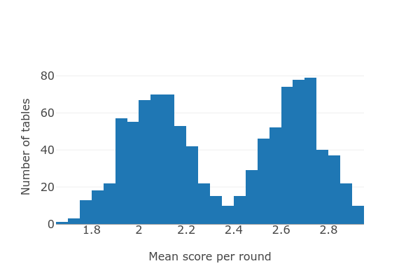
It looks like a mixture of two normal distributions centered at mean scores of 2.1 and 2.7. At this point, if I had to guess I would suspect that there's a single key whose contribution to the score is very important. To test how important a particular key is, we can take each position in the ID string and calculate the difference in mean score for those tables that had C and that position, and those that had D. Given a dict where the keys are the ID strings and the values are the scores, we can get list of all such differences:
def mean():
    ...

d = {
  'DDDCDCDDDCDDDDCCDCCDCCCDCDDDDCCDDDDDCCDCDCDCDDDCDDDDCDCDDCDDDCCD' : 2.0160,
  'CCDDCDDDCDDDDCDCCDDDCCCCCCCDCCDCCCCCDCDDDDCCDDDCCDCCDDDCCDDDCCCD' : 2.6258,
  ...
}

def get_diff(pos):
  c_score = mean([score for pattern, score in d.items() if pattern[pos] == 'C'])
  d_score = mean([score for pattern, score in d.items() if pattern[pos] == 'D'])
  return c_score - d_score

diffs = [get_diff(i) for i in range(64)]
and zip this together with our original list of lookup table keys to get a dict where the keys are the normal history tuples and the values are the differences. In other words, how much higher does a table score, on average, by having Cooperate as its response to a given set of conditions as opposed to Defect:
strings = [''.join(x) for x in itertools.product('CD', repeat=2)]
keys = sorted(list(itertools.product(strings,strings, strings)))
dict(zip(keys, diffs))

{
  ('CC', 'CC', 'CC'): 0.5985246110918112,
  ('CC', 'CC', 'CD'): -0.036229032273884965,
  ('CC', 'CC', 'DC'): 0.022587412332811585,
  ('CC', 'CC', 'DD'): 0.011773214960386635,
  ('CC', 'CD', 'CC'): 0.03782112365374468,
  ('CC', 'CD', 'CD'): 0.049968171759873226,
  ...
}
The crucially important key turns out to be the very first one: if the opponent started by cooperating twice, and both the opponent and me cooperated on both of the previous two turns, then cooperating again rather than defecting causes a massive score bonus of 0.6. This neatly explains the bimodal distribution that we saw in the histogram of scores. Intriguingly, the importance of following this rule almost completely disappears if the opponent started by doing something other than cooperating twice*:
{
  ('CC', 'CC', 'CC'): 0.5985246110918112,
  ...
  ('CD', 'CC', 'CC'): 0.008174615248195405,
  ...
  ('DC', 'CC', 'CC'): 0.01990436367685966,
  ...
  ('DD', 'CC', 'CC'): 0.007840839408610911,
}
Why is this one rule so important? It's probably something to do with the frequency with which the scenario occurs. In scoring 100 random tables, the pattern of mutual cooperation on two consecutive turns occurred just over 20 million times, while the next most common scenario - two consecutive turns of mutual defection - occurred about 7.5 million times. This is probably due to the presence in the Axelrod library of a large number of so-called nice strategies, i.e. those that will never defect before its opponent does. Note, however, that the importance of the double-mutual-cooperation pattern can't be due to frequency alone - while it occurs just over twice as often as double-mutual-defection, its scoring difference as measured in the dict above is about one hundred times greater.
The presence of nice strategies also neatly explains why the importance of responding correctly to double-mutual-cooperation goes away if the opponent defects any time in the first two turns. Given that our strategy always cooperates on the first two turns (regardless of what's in the lookup table), any opponent that defected on either of the first two turns is by definition not a nice strategy, so it's not so important for us to try to preserve a cycle of cooperation.
Looking at the results in this way is a bit unintuitive. We can visualize them better if we come up with short names for each of the four possibilities at each of the previous two turns. If both us and the opponent cooperated we'll call that mutual coop. If we both defected then we'll call it mutual defection. If we defected and the opponent cooperated (the best outcome for us) we'll call that betrayer. And if we cooperated but the opponent defected then we'll call that sucker*.
This gives us a dict that looks like this, where the two elements of the tuple in the key are the opponent's first two actions and the outcome of the last two turns:
{
  ...
  ('CC', 'betrayer-sucker'): -0.03,
  ...
}
So from the key/value pair in the example above if
- the opponent started by cooperating twice
- two turns ago we defected and the opponent cooperated (i.e. we were betrayer)
- in the last turn we cooperated and the opponent defected (i.e. we were the sucker)
then our average score will be 0.03 higher if we defect this turn rather than cooperating*.
Laying out the data like this allows us to draw a heatmap showing when it's better to cooperate and defect, and by how much:
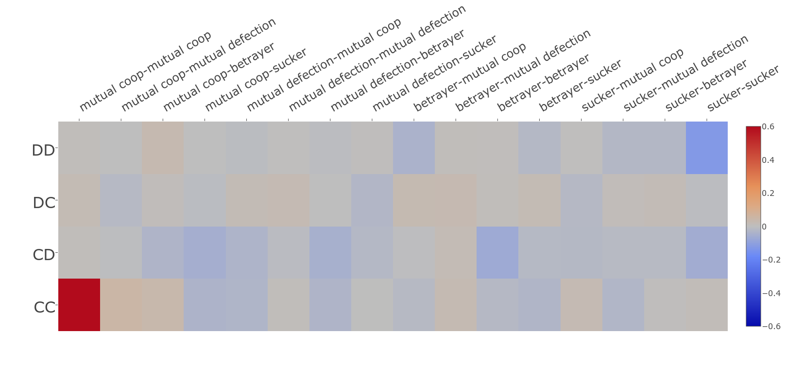
In this figure the opponent's first two actions are on the left side, and the sixteen possible outcomes of the previous two turns are arranged along the top. The colour of each square represents whether it's better to cooperate or defect, and by how much. Positive numbers (i.e. better to cooperate) are red, and the stronger the red colour the greater the increase in score given by cooperating. Negative numbers (i.e. better to defect) are blue. Positions for which there isn't much difference in score between defecting and cooperating show up in grey. The bar on the right-hand side gives the scale.
The most striking thing is the square in the bottom right corner, representing the case where the opponent started by cooperating twice and both previous turns have been mutual cooperation. This is the extremely strong benefit of not breaking cycles of mutual cooperation. The next strongest-coloured square is the top right, representing the situation where the opponent started by defecting twice, and on both previous turn we have been the sucker. In this scenario, it's much better to defect (blue) rather than cooperate.
The very high value in the bottom right makes it quite difficult to see the patterns in the data, because it's so much bigger than everything else. Let's get rid of those two very high value squares and redraw the figure, stretching the scale so we can see the other squares more clearly:
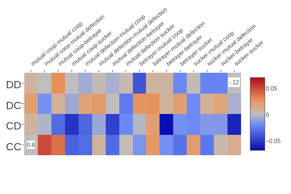
Notice how the colour scale has changed; pure red/blue now means a score of +0.06/-0.06. These numbers seem small, but remember that the current ten best strategies are separated by an average score of only 0.1.
This is a very interesting figure to look at, and I've spent quite a bit of time with it :-). The first thing that jumps out is just how different the patterns are for the different rows (i.e. how much the best thing to do in any given situation depends on the opponent's opening moves). Pretty much every column has one or two squares in it that are different to the others, sometimes with quite high scores. For example, look at the row corresponding to betrayer followed by mutual cooperation (ninth from the left). If the opponent started by defecting twice in a row, then it's a very good idea to defect (top row, a deep blue colour). But if the opponent started by defecting then cooperating, it's a very good idea to cooperate (second row, medium red).
The third row shows a surprising pattern: if the opponent started off by cooperating then defecting, then it's best to defect in every single scenario, except for two turns of mutual cooperation or betrayer followed by mutual defection*. Trying to come up with an explanation for all the patterns we see in this figure would be a long and tedious process, so let's move on.
Search method 2: pick the best action for each key independently
Studying this figure suggests an obvious approach to finding a high-scoring strategy: simply pick the action that maximizes the mean score at each position. If we have the differences stored in a dict as illustrated above, we can do this by just making a copy of the dict and then setting each value based on the sign of the score:
best_table = dict(key2diff)
for key, diff in sorted(key2diff.items()):
    if diff > 0:
        best_table[key] = 'C'
    else:
        best_table[key] = 'D'
This gives us a table with a score of around 2.95 - here it is on the chart from before (the new strategy is on the left):
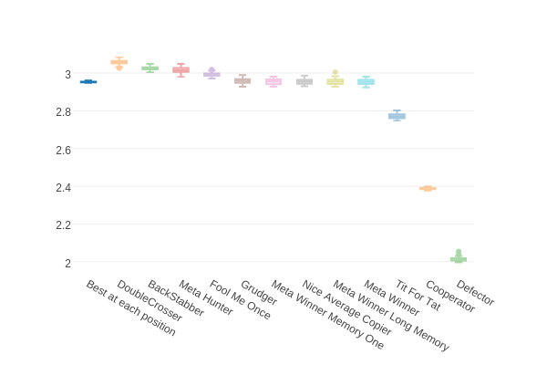
Notice that this strategy scores better than the best of our random 1000 strategies which we plotted on the histogram earlier: the best of those scored 2.93.
How likely is it that the lookup table chosen in this way is the best possible table? It depends on how much interaction there is between different keys. If our response to a particular scenario early in a match can affect the outcome of a different scenario later in a match, then we expect there to be subtle interactions between keys. We can tell just by browsing the strategies in the Axelrod library* that many of them do base their actions on what happened earlier in the match, so it's very likely that keys are not independent, and that we can find a better table with a different search method.
Search method 3: a greedy hill-climbing algorithm
Here's a slightly more sophisticated way of finding good strategies: a simple hill-climbing algorithm. We'll start with a random table, then repeatedly flip one of the keys at random and keep the new table if it's better:
current_table = get_random_table()
curent_score = axelrod_utils.do_table(current_table)[0]

for i in range(10000):
    # flip one key
    new_table = dict(current_table)
    key_to_change = random.choice(new_table.keys())
    new_table[key_to_change] = 'C' if new_table[key_to_change] == 'D' else 'D'

    new_score = axelrod_utils.do_table(new_table)[0]

    if new_score > curent_score:
        print("accepting change, new score is " + str(new_score))
        current_table = new_table
        curent_score = new_score
    else:
        print("rejecting change")

    with open("hillclimb.csv", 'a') as output:
        output.write(
            axelrod_utils.id_for_table(current_table)
            + ','
            + str(curent_score)
            + "\n")
This approach does pretty well; the best solution that it finds is comparable with DoubleCrosser with a mean score of around 3.1.
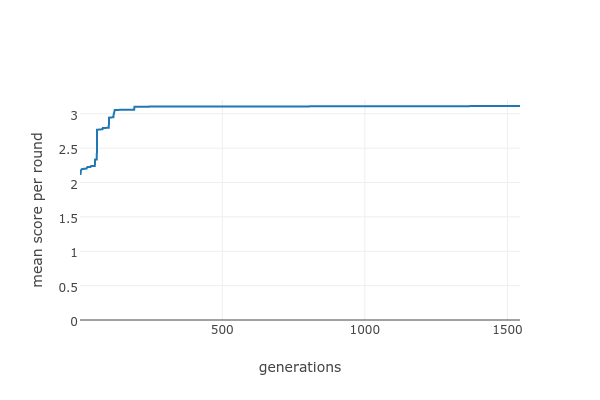
The score remains the same for long stretches, with only occasional jumps. We can try various things to fix it - how about flipping more than one key at a time?
for i in range(10000):
    new_table = dict(current_table)

    # flip several keys
    for j in range(10):
        key_to_change = random.choice(new_table.keys())
        new_table[key_to_change] = 'C' if new_table[key_to_change] == 'D' else 'Do'

    new_score = axelrod_utils.do_table(new_table)[0]
    ...
This doesn't make much difference, at least for this run:
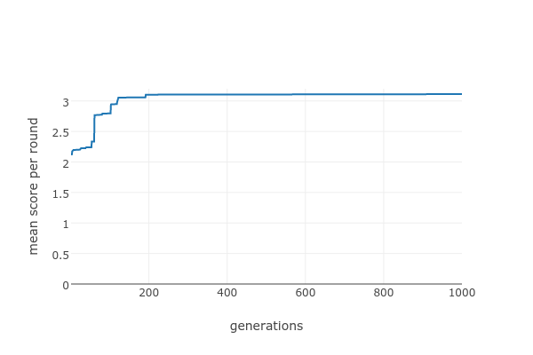
The problem with this approach (as with pretty much all naive hill-climbing algorithms) is that it's just too easy to get stuck in a local maximum: a pattern that's nowhere near the best, but where any small change is likely to make it worse.
If we wanted to pursue this hill-climbing idea further then we'd probably want to explore options like accepting changes that decrease the score with some probability, or starting with big changes (e.g. flipping half the keys) and making the changes smaller as we go on. We'd likely end up with something that resembled simulated annealing, or Monte Carlo sampling. However, we're not going to, because I want to talk about a completely different approach.
Search method four: an evolutionary algorithm
The idea behind an evolutionary algorithm is to find solutions to a complex, non-linear problem like ours by mimicking the process of natural selection. Rather than looking at a single lookup table at a time, we'll maintain a population of many lookup tables. In each generation, we'll mate pairs of tables to produce offspring that share properties of both (simulating the process of recombination) and also randomly flip some of the keys (simulating the process of mutation). We'll also throw in some more randomly-generated tables as a source of new variation. These processes will give us a bunch of new tables, which we'll calculate the scores for, and keep only the best individual tables for the next generation.
We can re-use large parts of the code we've already written* for the other search methods - we already know how to score a table and how to generate random tables. To "mate" two tables and produce a single offspring, we'll pick a random crossover point somewhere in the list of keys, and take the keys before that point from parent A and the keys after that point from parent B:
# assuming t1 and t2 are both valid lookup tables

crossover = random.randrange(len(t1.items()))

# the values (plays) for the offspring are copied from t1 up to the crossover point,
# and from t2 from the crossover point to the end
new_values = t1.values()[:crossover] + t2.values()[crossover:]

# turn those new values into a valid lookup table by copying the keys from t1 (the keys are the same for
# all tables, so it doesn't matter which one we pick)
new_table = dict(zip(t1.keys(), new_values))
To simulate mutation on a given table, we'll flip each key with a probability that we'll call the mutation rate:
# assuming c is a valid lookup table

# flip each value with a probability proportional to the mutation rate
for history, action in c.items():
    if random.random() < mutation_rate:
        c[history] = 'C' if action == 'D' else 'D'
For details of the rest of the algorithm see the repo here which also includes a command-line tool to run the evolutionary algorithm.
Here's the result of running the algorithm for around 200 generations:
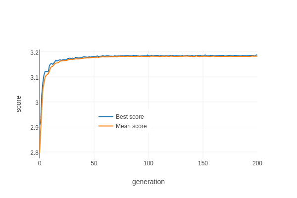
The blue line shows the score of the best table at each generation, the orange line shows the average score for the population. Compared to the other search methods we've tried, it finds good tables remarkably quickly. The first table that beats the current best strategy appears in the third generation with a score of 3.077, and the score levels out at around 3.185*.
Let's take a look at the winner. This next figure has two parts: on the top is the heatmap from before showing the differences we calculated from random tables, on the bottom is a similar chart showing the actions at each position for our winning table. The lower chart simply shows the action for each situation, so there are no shades of colour, only red and blue to indicate cooperation and defection. If a square in the bottom chart is the same colour as one in the top, it means that the action of our winning lookup table at that position is the same as the one we would have guessed based on random sampling.

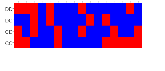
The patterns overlap somewhat, but there are some striking differences. This, along with the much higher score obtained by this table vs. simply picking the best option for each square independently, confirms our suspicion that there are complex interactions between the responses to different situations. It's tempting to pick out specific positions and try to come up with explanations for the rule, but confirming our guesses would involve looking in detail at the actual series of actions in the matches, so I will resist :-) except to note that the two squares with very strong scores in the heatmap - bottom left and top right - are the same.
Another way to look at the pattern of actions is to take each position, flip the action, and see how much worse the score is. Here's the heatmap:
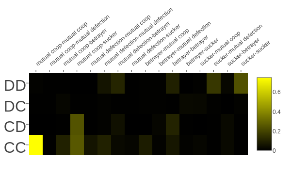
Note that we're not looking at the score for C versus D as we were before; instead we're looking at the reduction in score if we change the action at a particular position (I've changed the colour scale to reflect this). Brighter yellow means a bigger reduction in score. The top-right and bottom-left squares appear to be very important as we expect, but there are also some positions that seem a lot brighter than we'd expect based on the data from random tables. In particular, there are a couple of bright squares (i.e. a couple of important positions) showing that it's important to retaliate by defecting if we have just been suckered, at least for certain starting actions.
What we're really trying to do here is look at the relative contribution of different situations (keys in the lookup table dict) to getting a good score. The heatmap is kind of awkward for this, so let's try a different plot. Here's a scatter plot which shows, for each of our 64 keys, the advantage of C over D in the sample of random tables on the X axis and the advantage of C over D in the winning table:
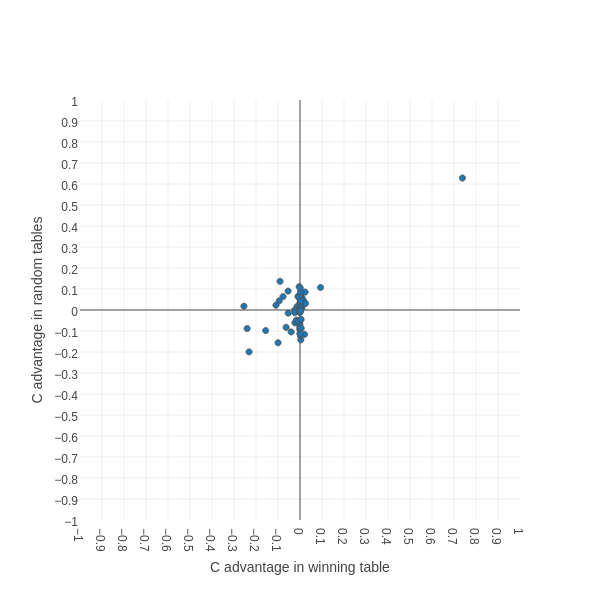
This plot takes a bit of interpretation....if a point is to the right of the vertical axis, it means that in the winning table we get a higher score if we have cooperate as the value. The further to the right it is, the greater the score. If a point is to the left of the vertical axis, then it's better to have defect as the value in the winning table. Points lying more or less on the vertical axis represent values that don't really affect the score for the winning table. The horizontal axis shows the same thing for the random tables: for points above the axis it's better to have cooperate, for points below it's better to have defect.
Way out on the top-right is our old friend representing the situation where the opponent started by cooperating twice and the last two turns were both mutual cooperation. We already know from the previous figures that, for both the random and winning tables, it's highly advantageous to have cooperate as our response. Interestingly, it's more advantageous for the winning table than for the random tables, possibly because the winning table tries* to maintain unbroken runs of mutual cooperation and so the situation simply occurs more often.
Let's zoom in on the middle bit of the chart, excluding this obvious outlier:
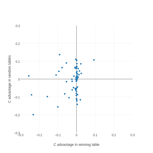
Quite a few interesting features become visible.
Firstly, there are many more points lying on or near the vertical axis than the horizontal axis. This means that there are many more keys whose value doesn't really matter for the winning table than for random tables. This makes intuitive sense; we would expect the winning table to try hard to avoid situations that are bad for it, so those situations will occur much more rarely for the winning table than for random tables, so the response to them won't be so important. When we look at the descriptions for these points, a lot of them seem to involve being the sucker, which we expect to be minimized by the winning table.
Secondly, there's generally a positive correlation - most of the points are in the top right quadrant (cooperation is advantageous in both the winning table and random tables) or the bottom right quadrant (defection is better in both the winning table and random tables).
Thirdly, there's a little cluster of points with quite strong scores in the top left quadrant. These represent situations where it's advantageous to cooperate in random tables, but advantageous to defect in the winning table. These are probably the most interesting points. For example, take the situation where the opponent started by cooperating twice, and the last two rounds have been mutual cooperation followed by sucker. In random tables, there's little systematic advantage to cooperating or defecting*; however in the winning table, there's a strong advantage to defecting.
Notably, there isn't a corresponding cluster in the bottom right quadrant (i.e. advantageous to defect in random tables but advantageous to cooperate in winning tables). In other words, there are situations where it's more advantageous to defect than we'd expect by looking at random tables, but there are none where it's more advantageous to cooperate. If you can think of a plausible reason for this, please leave a comment!
Anyway, here's the final box plot showing the new strategy (here labeled as LookerUp) along with the others from before:
Further work
There are a few obvious extensions to this idea. We could simply increase the memory depth of the table by, for instance, taking into account the last three turns rather than the last two. The problem with this is that we very quickly run into scaling issues: a lookup table with these dimensions will have 256 keys (four times as many as our current table), which means that the number of possible value patterns will be around 10^77, or around 10^57 times bigger than our current table. It's hard to see how the evolutionary algorithm could cope with that increase in search space.
Another idea would be to incorporate other information into the lookup table key. We could easily imagine, for example, a lookup table where the key includes the number of turns left in the match, or the total number of defections from the opponent. That leads to exactly the same kind of scaling problem, but worse!
Finally, it will be interesting to see how the winning pattern changes as new strategies are added to the Axelrod library. It's quite straightforwards, given enough cores, to re-run the evolutionary algorithm against new strategies, so the pattern for the winning strategy will continue to evolve in more ways than one.
 Subscribe to articles from the programming category via RSS or ATOM
Comments
comments powered by Disqus